What Type Of Variable Is Required When Drawing A Time-series Plot?

5 types of plots that will help you with time series analysis

And how to quickly create them using Python

While starting any project related to time series (and not only), one of the very first steps is to visualize the data. We do so to inspect the data we are dealing with and learn something about it, for example:

are there any patterns in the data?
are there any unusual observations (outliers)?
do the properties of the series of observations change over time (non-stationarity)?
are there any relationships between the variables?

And that is only the beginning. The characteristics of the d a ta that we learn from answering those questions should be then incorporated into the modeling approach we want to follow. Otherwise, we risk having a poor model that is not able to capture the special traits of the data we have. And as we learned time and time again — garbage in, garbage out.

In this article, I present a few types of plots that are very helpful while working with time series and briefly describe how we can interpret the results.

Setting up

Traditionally, we need to load all the required Python libraries. We do that in the following snippet.

Data

In this article, we will take a look at the famous Airline Passengers dataset, which you probably have already seen a few times in other articles or statistical handbooks/classes. It's very popular due to the simplicity of the observable patterns in it. That is also why it will serve its purpose well to illustrate different types of plots used for time series analysis.

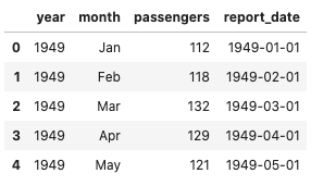
The dataset is also included in one of the plotting libraries we will use today — seaborn. We load the data by running the following lines. Additionally, we combine the year and month column to create a report_date field, which is a datatime.date object.

Examples of plots used for time series analysis

Having prepared the data, we will take a look at different types of plots used for time series analysis.

Time plots

A time plot is basically a line plot showing the evolution of the time series over time. We can use it as the starting point of the analysis to get some basic understanding of the data, for example, in terms of trend/seasonality/outliers, etc.

The easiest approach is to directly use the plot method of a pd.DataFrame.

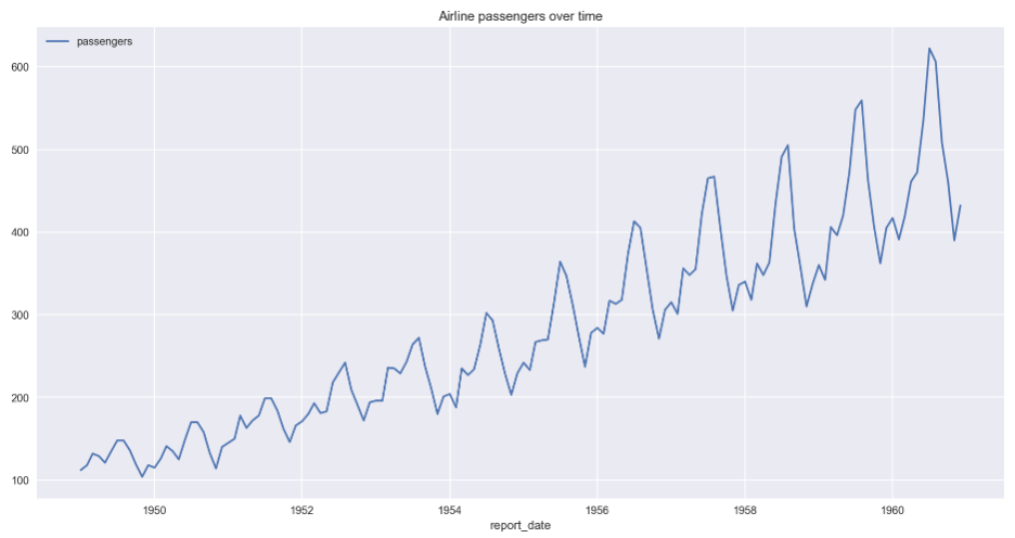
In the plot, we can observe an increasing trend over the years and clear seasonality in the form of the spikes during the summer months caused by vacation time.

The code could be further simplified by specifying the index of the DataFrame — then there is no need to specify the x axis. TIP: You can also change the default (matplotlib) backend of the plot method by running the following line:

          pd.options.plotting.backend = "plotly"

By doing so, you will generate the exact same plot as the one above, however, it will use plotly to make the plot interactive. Definitely helpful when you want to inspect particular observations or when you want to zoom in on a certain time period.

For completeness' sake, you can also easily use seaborn to generate the time plot:

In the past, there was a dedicated sns.tsplot function, however, it was deprecated in favor of the lineplot.

Seasonal plots

A seasonal plot is very similar to the time plot, with the exception that the data is plotted against the individual seasons. Choosing the definition of the season is up to the analyst and in our particular case, the season is simply the month. We can generate the seasonal plot by running the following code.

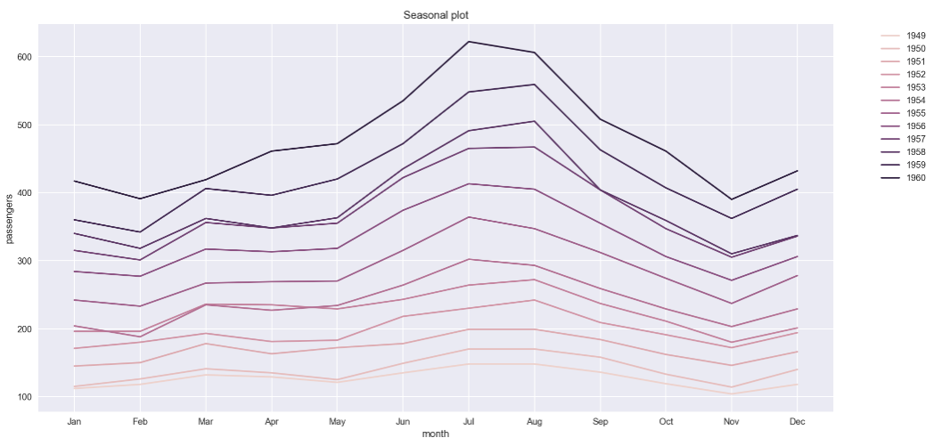
We can see that instead of plotting all 11 years as a one long series, we plot the same data per month. By doing so, we can clearly see the following:

the previously mentioned seasonal patterns with the spikes in summer months,
the trend, as the number of passengers is increasing yearly.

Additionally, a seasonal plot is especially useful for identifying the years in which the patterns change.

Alternatively, we can use a handy function from the statsmodels library to create a month_plot.

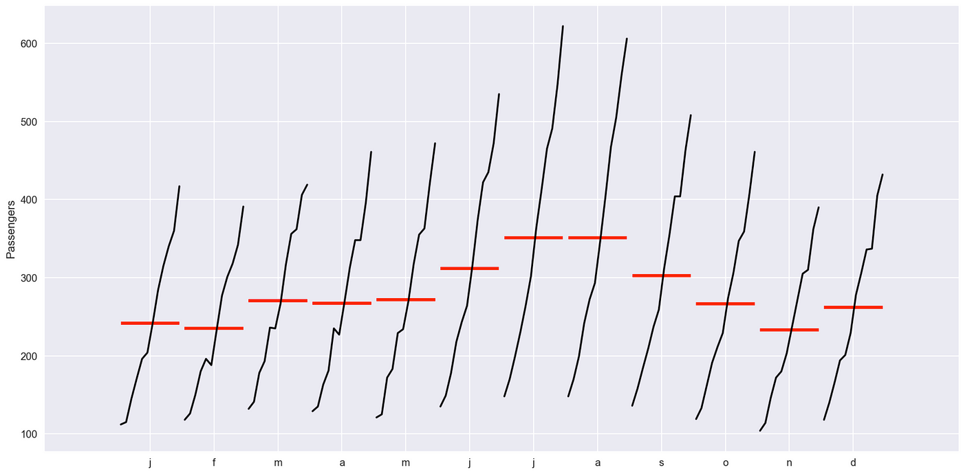
The information conveyed on this plot is very similar to the previous one, just the grouping is different. Aside from patterns over the years, we can also conveniently see the average values per month.

Lastly, we can also come up with a very similar plot, but this time per quarter. We only need to resample the data to quarterly frequency first and then use the quarter_plot function.

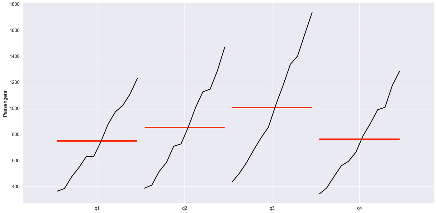
Polar seasonal plot

This is a variation of the seasonal plot, with the difference that it uses polar coordinates. Personally, I prefer the traditional seasonal plot, however, I am sure it is also useful for some specific cases.

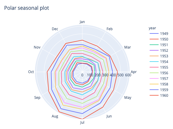
The very same plot could have been generated using matplotlib + seaborn, however, I try to follow the pragmatist approach. If it is possible to generate the plot much faster with a dedicated and well-established library such as plotly (or plotly_express), then I am strongly in favor of such a solution. And as an extra bonus we do get the interactivity for free!

Time series decomposition plot

Before actually showing the plot, I believe it makes sense to give a brief introduction to time series decomposition. In general, it provides a useful model for thinking about time series and facilitates a better understanding of the data. Decomposition assumes that a time series can be broken down into a combination of the following components:

level — the average value of the series,
trend — an increasing/decreasing pattern in the series,
seasonality — a repeating short-term cycle in the series,
noise — the random, unexplainable variation.

Where all time series have the level and noise components, while the trend and seasonality are optional.

What is left to add is that there are two main types of decomposition models:

additive — it assumes that the components above are added together (linear model). The changes over time are more or less constant.
multiplicative — it assumes that the components are multiplied by each other. Hence, the changes over time are non-linear and not constant, so they can increase/decrease with time. An example could be exponential growth.

With that much introduction, we can try an automatic decomposition approach. To do so, we use the seasonal_decompose function from the statsmodels library. For our case, when looking at the time plot we can see that there is monthly seasonality (12 periods, but that can be determined automatically given there is a timestamp index in the DataFrame) and the changes over time are not constant (increasing), so we will go with the multiplicative model.

In the plot we see the actual series in the first part, then the trend component, the seasonal one, and lastly the residuals (error term). The residuals close to 1 in the multiplicative model suggest a good fit. Bear in mind that they should be close to 0 for the additive one.

As always with automatic approaches, we should do a simple sanity check and do not trust the results blindly. For this simple example, we can see the confirmation of what we initially suspected about the time series.

Autocorrelation plots

When measuring the correlation between the time series and its lagged values (from previous points in time) we are talking about autocorrelation. There are two types of autocorrelation plots we can use.

The autocorrelation function (ACF) shows the value of the correlation coefficient between the series and its lagged values. The ACF considers all of the components of the time series (mentioned in the decomposition part) while finding the correlations. That is why it's known as the complete auto-correlation plot.

In contrast, the partial autocorrelation function (PACF) looks at the correlation between the residuals (the remainder after removing the effects explained by the previous lags) and the following lag value. This way, we effectively remove the already found variations before we find the next correlation. In practice, a high partial correlation indicates that there is some information in the residual that can be modeled by the next lag. So we might consider keeping that lag as a feature in our model.

We plot both ACF and PACF using the following snippet.

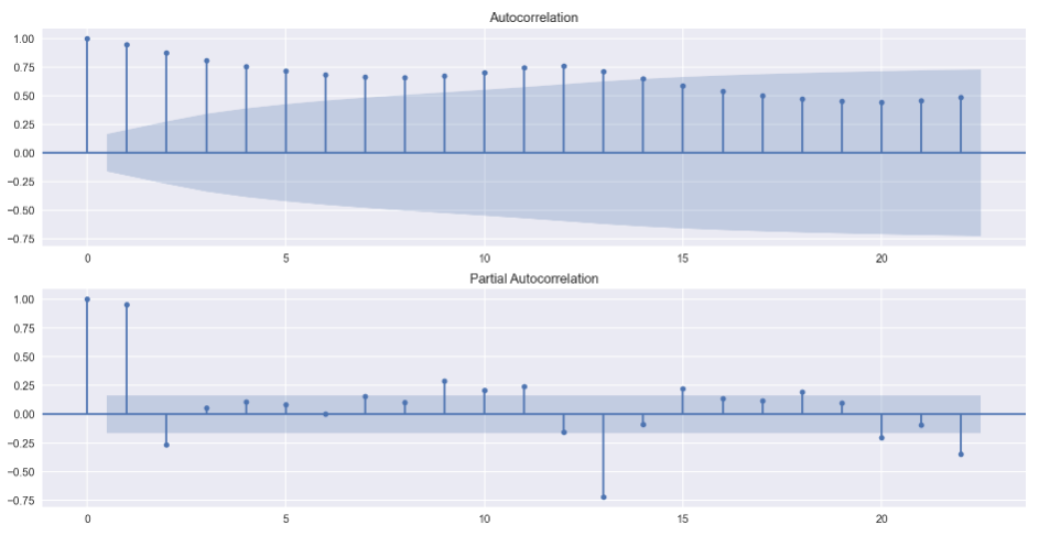
In the ACF plot, we can see that there are significant autocorrelations (above the 95% confidence interval, corresponding to the default 5% significance level). There are also some significant autocorrelations in the PACF plot.

Normally, the autocorrelations plots are often used for determining the stationarity of the time series or choosing the hyperparameters of the ARIMA class models, but these are topics for another article.

Conclusions

In this article, I showed 5 types of plots that will most likely come in handy while working with time series. The list is by no means exhaustive and often the choice of plots depends on the problem we are working on. For example, for stock price data we might want to visualize the candlestick chart instead of the regular time plot.

You can find the code used for this article on my GitHub. As always, any constructive feedback is welcome. You can reach out to me on Twitter or in the comments.